
Introduction
Small Area Estimation (SAE) encompasses statistical techniques designed to produce reliable estimates for sub-populations or geographical domains where sample sizes are too small for direct survey estimators to achieve acceptable precision.
The fastsae package provides high-performance C++
implementations (via Rcpp and RcppArmadillo)
for standard and advanced SAE models. It offers:
- Ultra-fast computation: Fisher-scoring and numerical solvers compiled in C++.
-
Exact numerical equivalence: Parameter estimates
and variance components match gold-standard implementations in the
saepackage to machine precision. -
Modern S3 interface: Seamless integration with
standard R methods (
summary(),coef(),fitted(),residuals(),autoplot()).
The Fay-Herriot Model
The area-level model introduced by Fay and Herriot (1979) links direct survey estimators with auxiliary variables :
where: -
represents domain-specific random effects. -
represents sampling errors with known sampling variance
(vardir).
The Empirical Best Linear Unbiased Predictor (EBLUP) is a weighted combination of the direct estimator and the regression-synthetic estimator:
where is the shrinkage factor ().
Step-by-Step Example
1. Load Package and Dataset
We use the built-in mys dataset (mean years of
schooling):
library(fastsae)
library(ggplot2)

data("mys")
head(mys)
#> # A tibble: 6 × 9
#>    area     y vardir   rse    x1    x2    x3      n  weight
#>   <int> <dbl>  <dbl> <dbl> <dbl> <dbl> <dbl>  <dbl>   <dbl>
#> 1     1  8.36  0.662  9.73   124    24    14  7280. 0.0326
#> 2     2  7.60  0.837 12.0     89    18     9  2743. 0.0123
#> 3     3  5.51  0.882 17.0     57    19     5  1706. 0.00764
#> 4     4  3.87  0.658 21.0     88    35    19  3073. 0.0138
#> 5     5  6.31  1.28  17.9    141    46    29 13400. 0.0600
#> 6     6  3.93  0.388 15.9     96    29    10  2004. 0.00897
2. Fit Fay-Herriot Model (eblup_fh)
To fit an area-level Fay-Herriot model using Restricted Maximum Likelihood (REML):
# Fit Fay-Herriot model
fit_fh <- eblup_fh(
  formula = y ~ x1 + x2 + x3,
  vardir = ~vardir,
  data = mys,
  method = "REML",
  print_result = FALSE
)
3. Model Summary and Coefficients
The standard S3 summary() method provides comprehensive
model diagnostics, variance components, and coefficient tests:
summary(fit_fh)
#>
#> ── Summary of fastsae Fit ──────────────────────────────────────────────────────
#> Call :
#> eblup_fh(formula = y ~ x1 + x2 + x3, vardir = ~vardir, data = mys, method =
#> "REML", print_result = FALSE)
#>
#> ✔ Convergence: Yes (in 6 iterations)
#> Model: Fay-Herriot (Area-level)
#> Method: eblup
#>
#> Variance Components:
#> sigma2_u: 2.608103
#>
#> Coefficients:
#>                   beta  std.error     zvalue pvalue
#> (Intercept)  3.1077510  0.7697687  4.0372527 0.0001
#> x1          -0.0019323  0.0098886 -0.1954019 0.8451
#> x2           0.0555184  0.0614129  0.9040187 0.3660
#> x3           0.0335344  0.0580013  0.5781663 0.5632
#>
#> Goodness of Fit:
#> loglikelihood           AIC           BIC
#>     -65.14251     140.28502     147.61370
#>
#> EBLUP Summary Statistics:
#>       mse              rse
#>  Min.   :0.2037   Min.   : 9.844
#>  1st Qu.:0.6886   1st Qu.:14.889
#>  Median :1.0156   Median :22.157
#>  Mean   :1.5434   Mean   :26.275
#>  3rd Qu.:2.4886   3rd Qu.:35.020
#>  Max.   :3.7074   Max.   :53.065
You can extract fixed-effects coefficients using
coef():
coef(fit_fh)
#>  (Intercept)           x1           x2           x3
#>  3.107750953 -0.001932259  0.055518370  0.033534410
Fitted EBLUP estimates and residuals can be extracted using standard generics:
4. Diagnostic Plots (autoplot)
fastsae extends ggplot2::autoplot() to
provide convenient diagnostic and comparison plots.
Direct Estimates vs EBLUP
Comparing the direct estimates against EBLUP demonstrates shrinkage towards the regression synthetic line:
autoplot(fit_fh, type = "estimates")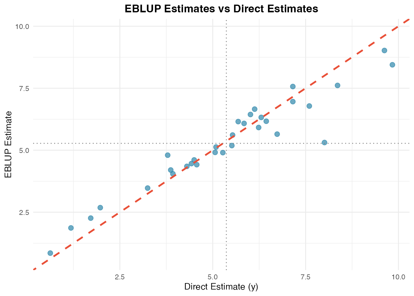
Mean Squared Error (MSE) Across Domains
Inspect domain-level uncertainty with MSE plots:
autoplot(fit_fh, type = "mse")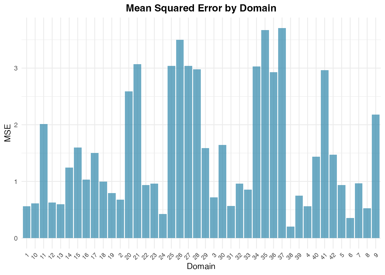
Exact Numerical Equivalence with sae
fastsae produces results that are mathematically
identical to sae::eblupFH:
if (requireNamespace("sae", quietly = TRUE)) {
  mys_clean <- as.data.frame(na.omit(mys))
  fit_fast <- eblup_fh(y ~ x1 + x2 + x3, vardir = ~vardir, data = mys_clean, print_result = FALSE)
  fit_sae <- sae::eblupFH(y ~ x1 + x2 + x3, vardir = vardir, data = mys_clean)

  # Check EBLUP estimates
  all.equal(fit_fast$df_eblup$eblup, as.vector(fit_sae$eblup))

  # Check regression coefficients
  all.equal(as.vector(coef(fit_fast)), as.vector(fit_sae$fit$estcoef$beta))

  # Check random effect variance (sigma2_u)
  all.equal(fit_fast$random_effect_var, fit_sae$fit$refvar)
}
#> [1] TRUE
Next Steps
Explore advanced modeling capabilities in fastsae: -
Spatial & Spatio-Temporal Models (EBLUP): spatial-temporal.html (SAR and AR(1)
dynamics). - Bayesian Area-Level SAE with INLA
(hb_area): hb-area-inla.html (Non-Gaussian families:
Beta, Poisson, Negative Binomial, Gamma, Binomial, and spatio-temporal
interactions). - Model Diagnostics and Residual Analysis
(diagnose): model-diagnostics.html (Calibration
tests, RSE reduction, and Moran’s I). - Unit-Level
Estimation: unit-level-bhf.html
(Battese-Harter-Fuller model).