Unit-Level Estimation with Battese-Harter-Fuller

Overview

Unlike area-level models that aggregate data prior to modeling, unit-level models operate directly on individual survey unit records (e.g., households, farms, or persons) while linking them to population auxiliary aggregates (e.g., census means or satellite imagery).

The fastsae package implements the nested error regression model of Battese, Harter, and Fuller (1988) via eblup_bhf(), providing fast estimation and parallel parametric bootstrap MSE.

Model Formulation

For individual unit $j$ ( $j = 1, \dots, n_d$ ) in small area $d$ ( $d = 1, \dots, D$ ):

$y_{dj} = x_{dj}^\top \beta + u_d + e_{dj}$

where: - $u_d \sim \text{i.i.d. } N(0, \sigma_u^2)$ is the area-specific random effect. - $e_{dj} \sim \text{i.i.d. } N(0, \sigma_e^2)$ is the unit-level error variance. - $u_d$ and $e_{dj}$ are mutually independent.

The small area population mean $\bar{Y}_d$ is estimated by:

$\hat{\bar{Y}}_d^{\text{EBLUP}} = \bar{X}_d^\top \hat{\beta} + \gamma_d (\bar{y}_d - \bar{x}_d^\top \hat{\beta})$

where: - $\bar{X}_d$ is the known population mean vector of auxiliary variables for domain $d$ . - $\bar{y}_d$ and $\bar{x}_d$ are the sample means for domain $d$ . - $\gamma_d = \frac{\sigma_u^2}{\sigma_u^2 + \sigma_e^2 / n_d}$ is the shrinkage ratio.

Step-by-Step Example

1. Data Preparation

We use the classic cornsoybean dataset, reporting corn crop hectares per segment in 12 Iowa counties:

library(fastsae)
data("cornsoybean")
data("cornsoybeanmeans")

# Align column names for population auxiliary means
df_pop <- cornsoybeanmeans
names(df_pop)[names(df_pop) == "MeanCornPixPerSeg"] <- "CornPix"
names(df_pop)[names(df_pop) == "MeanSoyBeansPixPerSeg"] <- "SoyBeansPix"
names(df_pop)[names(df_pop) == "CountyIndex"] <- "County"

head(cornsoybean)
#>   County CornHec SoyBeansHec CornPix SoyBeansPix
#> 1      1  165.76        8.09     374          55
#> 2      2   96.32      106.03     209         218
#> 3      3   76.08      103.60     253         250
#> 4      4  185.35        6.47     432          96
#> 5      4  116.43       63.82     367         178
#> 6      5  162.08       43.50     361         137
head(df_pop)
#>   County CountyName SampSegments PopnSegments CornPix SoyBeansPix
#> 1      1 CerroGordo            1          545  295.29      189.70
#> 2      2   Hamilton            1          566  300.40      196.65
#> 3      3      Worth            1          394  289.60      205.28
#> 4      4   Humboldt            2          424  290.74      220.22
#> 5      5   Franklin            3          564  318.21      188.06
#> 6      6 Pocahontas            3          570  257.17      247.13

2. Fit BHF Model with Bootstrap MSE

We fit the model using eblup_bhf(). To estimate domain-level Mean Squared Error (MSE), set compute_mse = TRUE:

fit_bhf <- eblup_bhf(
  formula = CornHec ~ CornPix + SoyBeansPix,
  unit_data = cornsoybean,
  Xpop = df_pop,
  domain_var = "County",
  popsize_var = "PopnSegments",
  method = "REML",
  compute_mse = TRUE,
  B = 50,
  seed = 123,
  print_result = FALSE
)
#> boundary (singular) fit: see help('isSingular')
#> boundary (singular) fit: see help('isSingular')
#> boundary (singular) fit: see help('isSingular')
#> boundary (singular) fit: see help('isSingular')
#> boundary (singular) fit: see help('isSingular')

summary(fit_bhf)
#> 
#> ── Summary of fastsae Fit ──────────────────────────────────────────────────────
#> Call :
#> eblup_bhf(formula = CornHec ~ CornPix + SoyBeansPix, unit_data = cornsoybean,
#> Xpop = df_pop, domain_var = "County", popsize_var = "PopnSegments", method =
#> "REML", B = 50, compute_mse = TRUE, seed = 123, print_result = FALSE)
#> 
#> ✔ Convergence: Yes (in - iterations)
#> Model: Battese-Harter-Fuller (Unit-level)
#> 
#> Variance Components:
#> sigma2_u: 63.3149 
#> 
#> Coefficients:
#>                  beta std.error    zvalue pvalue
#> (Intercept) 17.963979 30.974505  0.579960 0.5619
#> CornPix      0.366335  0.064959  5.639511 0.0000
#> SoyBeansPix -0.030364  0.067576 -0.449327 0.6532
#> 
#> EBLUP Summary Statistics:
#>       mse             rse       
#>  Min.   :24.89   Min.   :4.039  
#>  1st Qu.:36.74   1st Qu.:4.838  
#>  Median :46.45   Median :5.816  
#>  Mean   :49.96   Mean   :5.839  
#>  3rd Qu.:62.20   3rd Qu.:6.849  
#>  Max.   :81.65   Max.   :7.921

3. Inspect Domain Estimates

The resulting df_eblup data frame contains the domain estimates along with sample size, MSE, and Relative Standard Error (RSE):

head(fit_bhf$df_eblup)
#>   domain    eblup samp_size      mse      rse
#> 1      1 122.5825         1 81.64650 7.371235
#> 2      2 123.5274         1 69.94384 6.770354
#> 3      3 113.0343         1 80.17283 7.921429
#> 4      4 114.9901         2 52.75789 6.316599
#> 5      5 137.2660         3 32.60240 4.159698
#> 6      6 108.9807         3 59.61422 7.084763

4. Visualizing Results with `autoplot`

For unit-level models, domain uncertainty and model comparisons can be displayed with autoplot():

# Plot MSE across counties
autoplot(fit_bhf, type = "mse")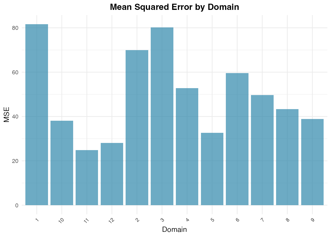


# Plot EBLUP estimates with confidence intervals
autoplot(fit_bhf, type = "comparison")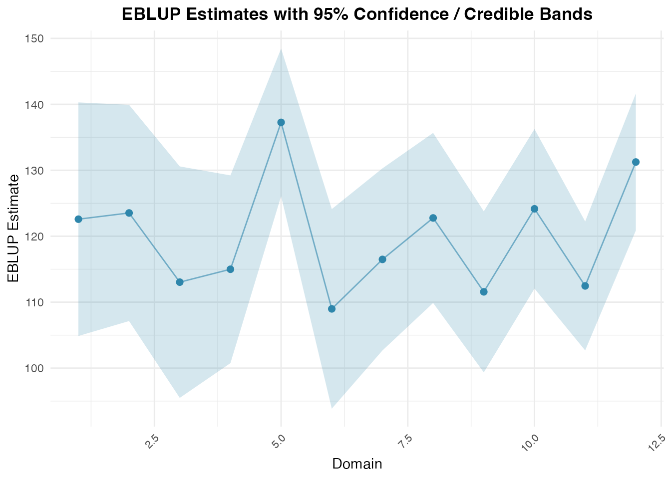

References

Battese, G. E., Harter, R. M., & Fuller, W. A. (1988). An error-components model for prediction of county crop areas using survey and satellite data. Journal of the American Statistical Association, 83(401), 28–36.
Rao, J. N. K., & Molina, I. (2015). Small Area Estimation (2nd ed.). John Wiley & Sons.