Spatial and Spatio-Temporal Models

Overview

When small areas are geographic units (such as counties, regencies, or districts), spatial correlation frequently occurs: neighboring areas tend to have more similar outcomes than distant ones. Furthermore, when surveys are repeated over multiple years, temporal correlation between time periods is also present.

fastsae provides specialized, high-performance implementations for both: 1. Spatial Fay-Herriot (eblup_sfh): Simultaneous Autoregressive SAR(1) random effects. 2. Spatio-Temporal Fay-Herriot (eblup_stfh): Combined spatial SAR(1) and temporal AR(1) random effects.

---

1. Spatial Fay-Herriot Model (eblup_sfh)

Model Formulation

The Spatial Fay-Herriot model (Pratesi & Salvati, 2008) models area random effects using a Simultaneous Autoregressive (SAR(1)) process:

$$y = X\beta + u + e$$

$$u = \rho_1 W u + \epsilon_1 \implies u = (I - \rho_1 W)^{-1} \epsilon_1$$

where: - $W$ is a known row-standardized spatial proximity matrix ($D \times D$). - $\rho_1 \in (-1, 1)$ is the spatial autoregressive parameter. - $\epsilon_1 \sim N(0, \sigma_{u1}^2 I_D)$ is independent innovation noise. - $e \sim N(0, V_e)$ is sampling error with diagonal matrix $V_e = \text{diag}(D_1, \dots, D_D)$.

Fitting the Model

library(fastsae)
data("mys")
data("mys_proxmat")

# Fit Spatial Fay-Herriot model with REML
fit_sfh <- eblup_sfh(
  formula = y ~ x1 + x2 + x3,
  vardir = ~vardir,
  data = mys,
  W = mys_proxmat,
  method = "REML",
  print_result = FALSE
)

summary(fit_sfh)
#> 
#> ── Summary of fastsae Fit ──────────────────────────────────────────────────────
#> Call :
#> eblup_sfh(formula = y ~ x1 + x2 + x3, vardir = ~vardir, data = mys, method =
#> "REML", W = mys_proxmat, print_result = FALSE)
#> 
#> ✔ Convergence: Yes (in 8 iterations)
#> Model: Spatial Fay-Herriot (Area-level SAR)
#> Method: REML
#> 
#> Variance & Correlation Components:
#>  parameter  estimate std.error
#>   sigma2_u  1.493692  1.095052
#>        rho -1.000000 10.836726
#> rho (spatial): -1 
#> 
#> Coefficients:
#>                    beta   std.error      zvalue pvalue
#> (Intercept)  3.03659649  0.62669962  4.84537788 0.0000
#> x1          -0.00085935  0.00824230 -0.10426151 0.9170
#> x2           0.04983809  0.05273618  0.94504545 0.3446
#> x3           0.03929798  0.05006522  0.78493574 0.4325
#> 
#> Goodness of Fit:
#> loglikelihood           AIC           BIC 
#>     -65.02194     142.04389     150.83830 
#> 
#> EBLUP Summary Statistics:
#>       mse              rse        
#>  Min.   :0.1936   Min.   : 9.512  
#>  1st Qu.:0.5725   1st Qu.:13.224  
#>  Median :0.8264   Median :19.840  
#>  Mean   :1.0470   Mean   :21.974  
#>  3rd Qu.:1.3772   3rd Qu.:30.137  
#>  Max.   :2.3507   Max.   :45.188

Unsampled Domains and Spatial Kriging

A major advantage of eblup_sfh in fastsae is its automatic handling of unsampled domains (domains with y = NA). Instead of throwing an error or requiring manual subsetting, eblup_sfh automatically performs full-spatial kriging:

# Count sampled vs unsampled domains
table(is.na(mys$y))
#> 
#> FALSE  TRUE 
#>    32    10

# Inspect estimates for unsampled domains
head(fit_sfh$df_eblup[is.na(mys$y), ])
#>    domain  y vardir    eblup random_effect      mse      rse
#> 21     21 NA      0 3.660260             0 1.904961 37.70779
#> 25     25 NA      0 4.153888             0 1.862352 32.85309
#> 26     26 NA      0 5.305132             0 2.206307 27.99863
#> 27     27 NA      0 4.300605             0 1.872941 31.82237
#> 28     28 NA      0 5.039354             0 1.824374 26.80292
#> 34     34 NA      0 3.491430             0 1.853401 38.99253

For unsampled areas, prediction borrows strength from both the regression synthetic component $x_d^\top \hat{\beta}$ and spatial proximity to neighboring sampled areas through $(I - \hat{\rho}_1 W)^{-1}$.

Multi-Threaded Bootstrap MSE

In addition to analytical Prasad-Rao style MSE, eblup_sfh supports multi-threaded OpenMP bootstrap MSE estimation:

• Parametric Bootstrap (mse_method = "pbmse")
• Non-Parametric Bootstrap (mse_method = "npbmse")

fit_sfh_pb <- eblup_sfh(
  formula = y ~ x1 + x2 + x3,
  vardir = ~vardir,
  data = mys,
  W = mys_proxmat,
  mse_method = "pbmse",
  B = 50,
  n_threads = 2,
  seed = 123,
  print_result = FALSE
)
#> ℹ 10 unsampled domain(s) detected. Bootstrap MSE (pbmse) is computed for the 32 sampled domain(s); unsampled domain(s) get a full-spatial synthetic (kriging) prediction and analytical MSE instead.

head(fit_sfh_pb$df_eblup[, c("domain", "y", "eblup", "mse", "mse_pb", "mse_pbbc")])
#>   domain        y    eblup       mse    mse_pb  mse_pbbc
#> 1      1 8.359527 7.282308 0.4797992 0.5043246 0.6019482
#> 2      2 7.599650 6.423856 0.6156692 0.4362874 0.6860557
#> 3      3 5.514137 5.023421 0.5519476 0.6400385 0.7173447
#> 4      4 3.869326 4.324716 0.4811841 0.4962733 0.5593804
#> 5      5 6.305063 6.344991 0.7315241 0.5816691 0.8868638
#> 6      6 3.926807 4.087497 0.3403445 0.4636404 0.3729264

---

2. Spatio-Temporal Fay-Herriot Model (eblup_stfh)

Model Formulation

The Spatio-Temporal model (Marhuenda, Molina, & Morales, 2013) combines spatial correlation and temporal autoregression across a balanced panel of $D$ areas observed over $T$ time periods:

$$y_{dt} = x_{dt}^\top \beta + u_{1d} + u_{2dt} + e_{dt}$$

where: - $u_1 = (u_{11}, \dots, u_{1D})^\top$ captures static spatial effects: $u_1 = \rho_1 W u_1 + \epsilon_1$. - $u_{2d} = (u_{2d1}, \dots, u_{2dT})^\top$ captures dynamic temporal effects for area $d$: $u_{2dt} = \rho_2 u_{2d,t-1} + \epsilon_{2dt}$. - $e_{dt} \sim \text{ind. } N(0, D_{dt})$ are sampling errors.

Fitting the Spatio-Temporal Model

data("mys_panel")

# Prepare balanced panel without missing values
panel_data <- mys_panel[!is.na(mys_panel$y) & mys_panel$year >= 2024, ]
W_sub <- mys_proxmat[-c(21, 25), -c(21, 25)]

# Fit Spatio-Temporal model with bootstrap MSE
fit_stfh <- eblup_stfh(
  formula = y ~ x1 + x2 + x3,
  data = panel_data,
  vardir = ~vardir,
  domain = ~area,
  time = ~year,
  W = W_sub,
  model = "ST",
  compute_mse = TRUE,
  B = 25,
  seed = 42,
  print_result = FALSE
)

summary(fit_stfh)
#> 
#> ── Summary of fastsae Fit ──────────────────────────────────────────────────────
#> Call :
#> eblup_stfh(formula = y ~ x1 + x2 + x3, vardir = ~vardir, data = panel_data,
#> domain = ~area, time = ~year, W = W_sub, model = "ST", compute_mse = TRUE, B =
#> 25, seed = 42, print_result = FALSE)
#> 
#> ✔ Convergence: Yes (in 12 iterations)
#> Model: Spatio-Temporal Fay-Herriot (ST-FH)
#> Method: REML
#> 
#> Variance & Correlation Components:
#>    estimate  std.error
#>   0.0000000  3.3656683
#>  -0.9990000 10.2860936
#>   2.2451375  0.7260280
#>   0.5738458  0.4727148
#> 
#> Coefficients:
#>                   beta  std.error     zvalue pvalue
#> (Intercept)  3.7498891  0.4538487  8.2624211 0.0000
#> x1          -0.0053032  0.0046392 -1.1431391 0.2530
#> x2           0.0606926  0.0258702  2.3460387 0.0190
#> x3           0.0173309  0.0257334  0.6734780 0.5006
#> 
#> Goodness of Fit:
#>   loglike       AIC       BIC 
#> -243.6043  503.2087  525.5086 
#> 
#> EBLUP Summary Statistics:
#>       mse              rse         
#>  Min.   :0.1885   Min.   :  7.866  
#>  1st Qu.:0.5410   1st Qu.: 12.858  
#>  Median :0.7642   Median : 15.707  
#>  Mean   :0.8911   Mean   : 20.922  
#>  3rd Qu.:1.0287   3rd Qu.: 19.913  
#>  Max.   :3.2885   Max.   :276.605

The estimated variance and correlation components include: - sigma21: Spatial random effect variance ($\sigma_{u1}^2$). - rho1: Spatial autocorrelation ($\rho_1$). - sigma22: Temporal random effect variance ($\sigma_{u2}^2$). - rho2: Temporal AR(1) autoregression coefficient ($\rho_2$).

---

3. Comparing Models with autoplot

You can directly compare EBLUP estimates and uncertainty across different models using autoplot():

# Compare Fay-Herriot vs Spatial Fay-Herriot
fit_fh <- eblup_fh(y ~ x1 + x2 + x3, vardir = ~vardir, data = na.omit(mys), print_result = FALSE)
W_clean <- mys_proxmat[!is.na(mys$y), !is.na(mys$y)]
fit_sfh_clean <- eblup_sfh(y ~ x1 + x2 + x3, vardir = ~vardir, data = na.omit(mys), W = W_clean, print_result = FALSE)

autoplot(list("Standard FH" = fit_fh, "Spatial FH" = fit_sfh_clean), type = "comparison")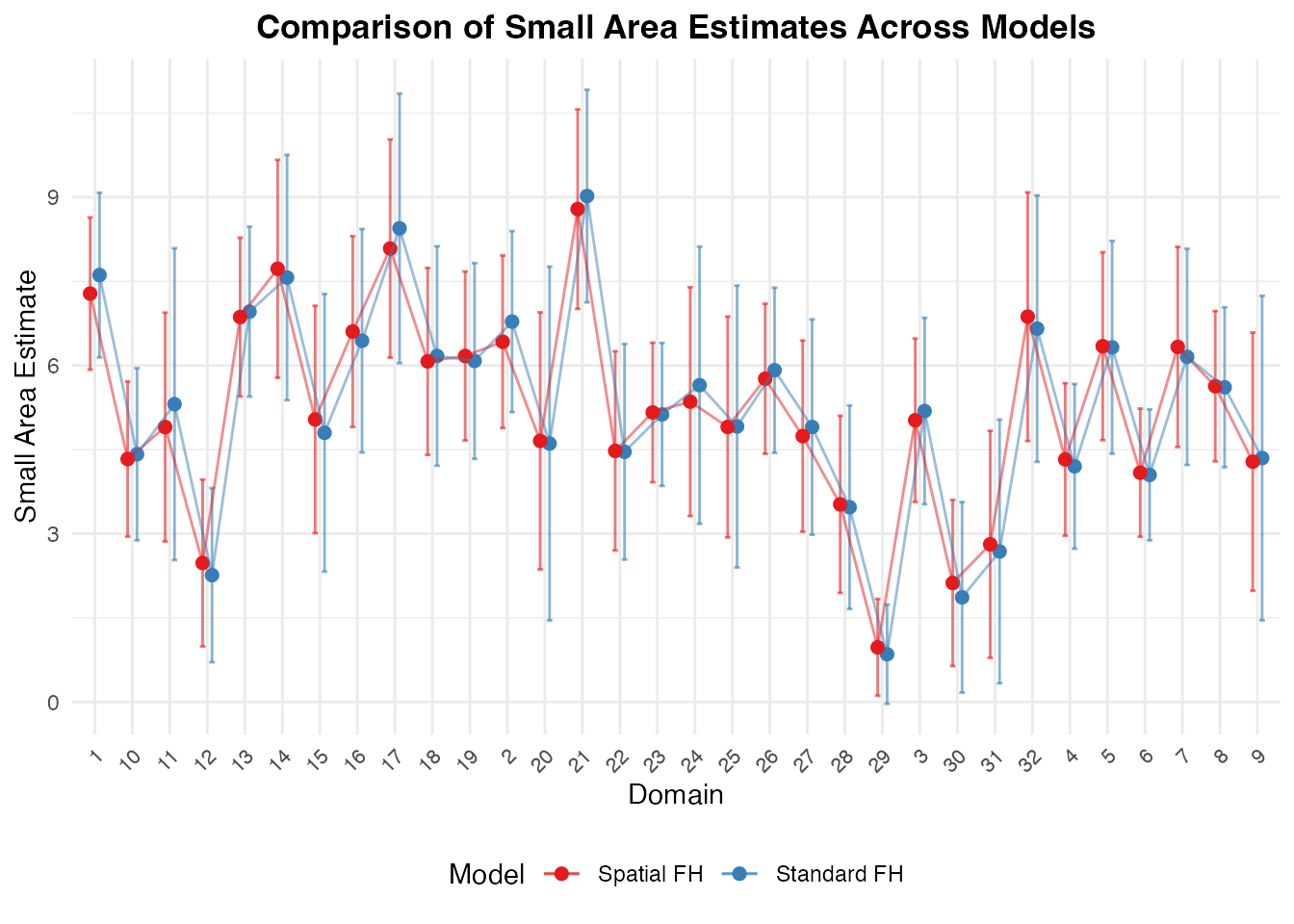

---

4. Bayesian Spatio-Temporal Modeling (hb_area)

In addition to frequentist C++ EBLUP implementations (eblup_sfh and eblup_stfh), fastsae provides hb_area() for Bayesian spatio-temporal modeling powered by INLA. This supports: - Bounded proportions via Beta regression (matching tipsae) - Discrete counts via Poisson and Negative Binomial regression - Binary aggregates via Binomial regression - Flexible space-time structures including domain-specific random walks, separable dynamic fields, and Knorr-Held Types I–IV.

For full details and a case study on Italian poverty data, see the vignette Bayesian Area-Level Small Area Estimation with INLA.

---

References

• Marhuenda, Y., Molina, I., & Morales, D. (2013). Small area estimation with spatio-temporal Fay-Herriot models. Computational Statistics & Data Analysis, 58, 308–325.
• Pratesi, M., & Salvati, N. (2008). Small area estimation for spatially correlated data: A Fay-Herriot with the spatial linear spline model. Journal of Applied Statistics, 35(7), 781–794.