Creates diagnostic and comparison plots for Small Area Estimation (SAE)
models fitted with fastsae. This extends the generic
autoplot from ggplot2.
Arguments
- object
An object of class
fastsae, or a (named) list offastsaeobjects.- type
Type of plot to create.
For a single
fastsaeobject:"comparison","ribbon","mse","estimates","scatter","rse", or"map".For a list of
fastsaeobjects:"comparison","mse","scatter", or"map".
- ...
Additional arguments passed to internal plotting helpers (e.g.
title) or to ggplot2 layers.
Examples
library(fastsae)
# Single model plot
fit_fh <- eblup_fh(y ~ x1 + x2 + x3, data = mys, vardir = "vardir")
#>
#> ── Fast Small Area Estimation (fastsae) ────────────────────────────────────────
#> Call:
#> eblup_fh(formula = y ~ x1 + x2 + x3, vardir = "vardir", data = mys)
#>
#> ✔ Convergence: Yes (in 6 iterations)
#> Model: Fay-Herriot (Area-level)
#> Method: eblup
#> Random effect variance (sigma2_u): 2.608103
#>
#> Fixed Effects Coefficients:
#> beta std.error zvalue pvalue
#> (Intercept) 3.1077510 0.7697687 4.0372527 0.0001
#> x1 -0.0019323 0.0098886 -0.1954019 0.8451
#> x2 0.0555184 0.0614129 0.9040187 0.3660
#> x3 0.0335344 0.0580013 0.5781663 0.5632
#>
#> EBLUP Estimates (First 6 domains):
#> domain y eblup vardir random_effect mse rse
#> 1 1 8.359527 7.612738 0.6618838 2.94266461 0.5616180 9.844182
#> 2 2 7.599650 6.782316 0.8374691 2.54539588 0.6784873 12.144869
#> 3 3 5.514137 5.187060 0.8822257 0.96692722 0.7190378 16.347620
#> 4 4 3.869326 4.201545 0.6581716 -1.31646412 0.5619314 17.841554
#> 5 5 6.305063 6.323679 1.2788021 -0.03796677 0.9370273 15.307573
#> 6 6 3.926807 4.048590 0.3878004 -0.81904048 0.3548310 14.713194
#> ... and 36 more rows.
#>
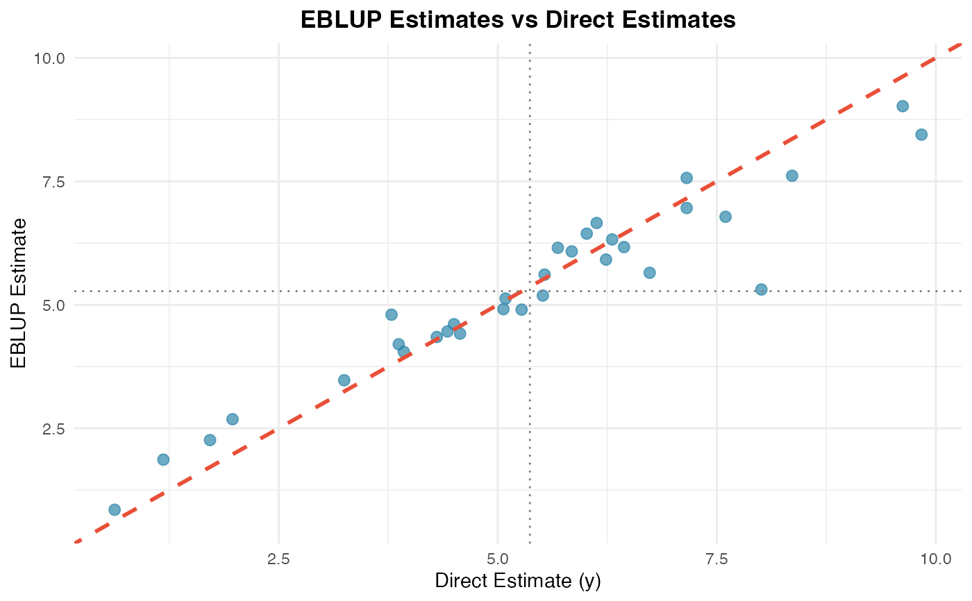
autoplot(fit_fh, type = "estimates")
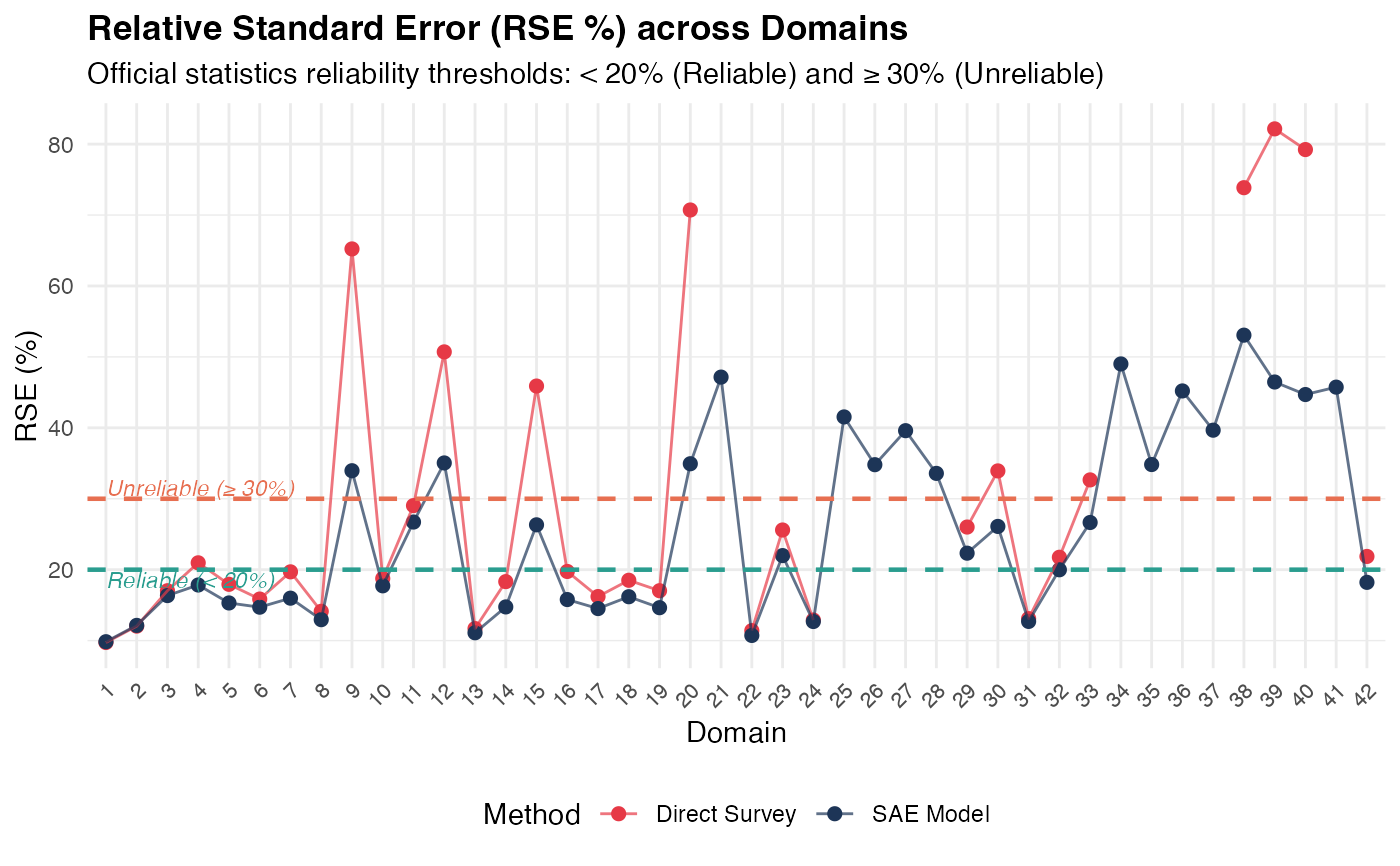
 autoplot(fit_fh, type = "rse")
#> Warning: Removed 10 rows containing missing values or values outside the scale range
#> (`geom_point()`).
autoplot(fit_fh, type = "rse")
#> Warning: Removed 10 rows containing missing values or values outside the scale range
#> (`geom_point()`).
 # Compare two models
fit_sfh <- eblup_sfh(y ~ x1 + x2 + x3, data = mys, vardir = "vardir", W = mys_proxmat)
#>
#> ── Fast Small Area Estimation (fastsae) ────────────────────────────────────────
#> Call:
#> eblup_sfh(formula = y ~ x1 + x2 + x3, vardir = "vardir", data = mys, W =
#> mys_proxmat)
#>
#> ✔ Convergence: Yes (in 8 iterations)
#> Model: Spatial Fay-Herriot (Area-level SAR)
#> Method: REML
#> Random effect variance (sigma2_u): 1.493692
#> Spatial autocorrelation (rho): -1
#>
#> Fixed Effects Coefficients:
#> beta std.error zvalue pvalue
#> (Intercept) 3.03659649 0.62669962 4.84537788 0.0000
#> x1 -0.00085935 0.00824230 -0.10426151 0.9170
#> x2 0.04983809 0.05273618 0.94504545 0.3446
#> x3 0.03929798 0.05006522 0.78493574 0.4325
#>
#> EBLUP Estimates (First 6 domains):
#> domain y vardir eblup random_effect mse rse
#> 1 1 8.359527 0.6618838 7.282308 2.605985416 0.4797992 9.511756
#> 2 2 7.599650 0.8374691 6.423856 2.212974942 0.6156692 12.214562
#> 3 3 5.514137 0.8822257 5.023421 0.892393688 0.5519476 14.789360
#> 4 4 3.869326 0.6581716 4.324716 -1.127251956 0.4811841 16.039766
#> 5 5 6.305063 1.2788021 6.344991 -0.002629647 0.7315241 13.479795
#> 6 6 3.926807 0.3878004 4.087497 -0.704885769 0.3403445 14.272560
#> ... and 36 more rows.
#>
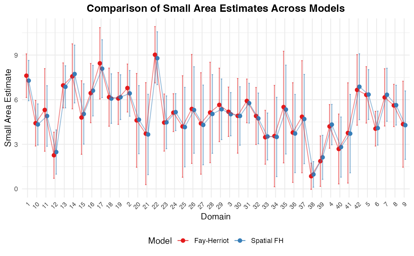
autoplot(list("Fay-Herriot" = fit_fh, "Spatial FH" = fit_sfh), type = "comparison")
# Compare two models
fit_sfh <- eblup_sfh(y ~ x1 + x2 + x3, data = mys, vardir = "vardir", W = mys_proxmat)
#>
#> ── Fast Small Area Estimation (fastsae) ────────────────────────────────────────
#> Call:
#> eblup_sfh(formula = y ~ x1 + x2 + x3, vardir = "vardir", data = mys, W =
#> mys_proxmat)
#>
#> ✔ Convergence: Yes (in 8 iterations)
#> Model: Spatial Fay-Herriot (Area-level SAR)
#> Method: REML
#> Random effect variance (sigma2_u): 1.493692
#> Spatial autocorrelation (rho): -1
#>
#> Fixed Effects Coefficients:
#> beta std.error zvalue pvalue
#> (Intercept) 3.03659649 0.62669962 4.84537788 0.0000
#> x1 -0.00085935 0.00824230 -0.10426151 0.9170
#> x2 0.04983809 0.05273618 0.94504545 0.3446
#> x3 0.03929798 0.05006522 0.78493574 0.4325
#>
#> EBLUP Estimates (First 6 domains):
#> domain y vardir eblup random_effect mse rse
#> 1 1 8.359527 0.6618838 7.282308 2.605985416 0.4797992 9.511756
#> 2 2 7.599650 0.8374691 6.423856 2.212974942 0.6156692 12.214562
#> 3 3 5.514137 0.8822257 5.023421 0.892393688 0.5519476 14.789360
#> 4 4 3.869326 0.6581716 4.324716 -1.127251956 0.4811841 16.039766
#> 5 5 6.305063 1.2788021 6.344991 -0.002629647 0.7315241 13.479795
#> 6 6 3.926807 0.3878004 4.087497 -0.704885769 0.3403445 14.272560
#> ... and 36 more rows.
#>
autoplot(list("Fay-Herriot" = fit_fh, "Spatial FH" = fit_sfh), type = "comparison")